In order for the robot to perform autonomous tasks we need a way to instruct the robot to follow a precise path. To accomplish this we use a technique called Pure Pursuit which described in this white paper by R. Craig Coulter.
The basic idea behind Pure Pursuit path following is that at any given point in time we find the point on the desired path that is closest to the current robot’s position. We then look ahead on the path a certain distance and attempt to steer the robot to that position.
The Achilles heel of this technique is that we need to be able to keep track of the robots absolute position on the field. As it turns out, this is actually quite hard to do.
To accomplish this tracking, we use the encoders on the drive wheels and a gyro to integrate the robot’s position over time. Periodically we get the current value of the drive wheel encoders and the gyro, and using this information and a little trigonometry compute the change in x and y during that interval. The problem with this is that we get an accumulated error which increases over time which can end up with fairly large error. However, we are able to get the robot to follow fairly complex paths reasonably reliably, at least for a short time.
Since doing these calculation requires precise timing, for the NerfBot, we are using an Arduino based module to read the encoders and gyro and compute the position.
Now in order for this all to work, we must have a reasonable path for the robot to follow. To define our paths we use 5th order Bezier curves and then compute paths for the left wheel, robot center and right wheel simultaneously so as to ensure that neither the left or right speeds exceeded whatever maximum velocity is set. The tool we will use to design these paths is called PathPlanner and can be found in the PiUtil folder of the RobotTools2021 that you have installed.
The paths are constructed by a series of 5th order Bezier curves. The parametric curve is defined by 6 control points, P0, P1, P2, P3, P4 and P5. Only the first and last points lie on the curve, the other points control the shape of the curve.
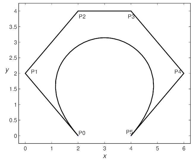
When two curves of the path are joined, we want the slope (i.e. first derivative) of the curves to match. To achieve this we find that the last two points of the first curve (P4 and P5) must be co-linear with the first two points of the next curve (P0 and P1). In addition, we need the velocity of the left and right wheels to be continuous as well. In order to achieve this, the second derivative of the curves must also match at the join point. This requires that the last 3 points of the first curve (P3, P4, and P5) be co-linear with the first three points of the second curve (P0, P1, and P2). This constrains our choices for the values of the control points but still gives us the ability control the shape of the curves.
Running the PathPlanner program from the PiUtils folder should produce the following:
The fields in the lower left have the following meanings:
- # Points – Specifies the number of points that should be generated along each Bezier curve. 1000 is a reasonable number here.
- DT – Specifies the time between points generated for the final output
- Max Velocity – Specifies the default maximum velocity for the robot in feet/sec.
- Max Accel – Specifies the maximum acceleration for the robot in feet/sec*sec.
- Max Decel – Specifies the maximum deceleration for the robot in feet/sec*sec.
- Max Jerk – Specifies the maximum jerk for the robot in feet/sec*sec*sec.
- Wheel Base – Specifies the distance between the drive wheels of the tank drive robot in feet.
In the Waypoints edit field we will enter the waypoints of our path. There are a number of formats for these values. The simplest consists of the starting point, angle in the following format:
x, y, angle
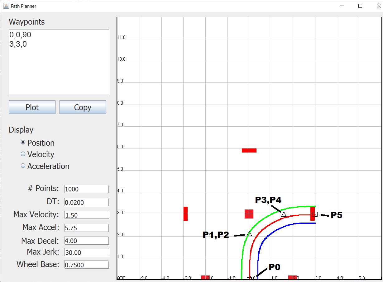
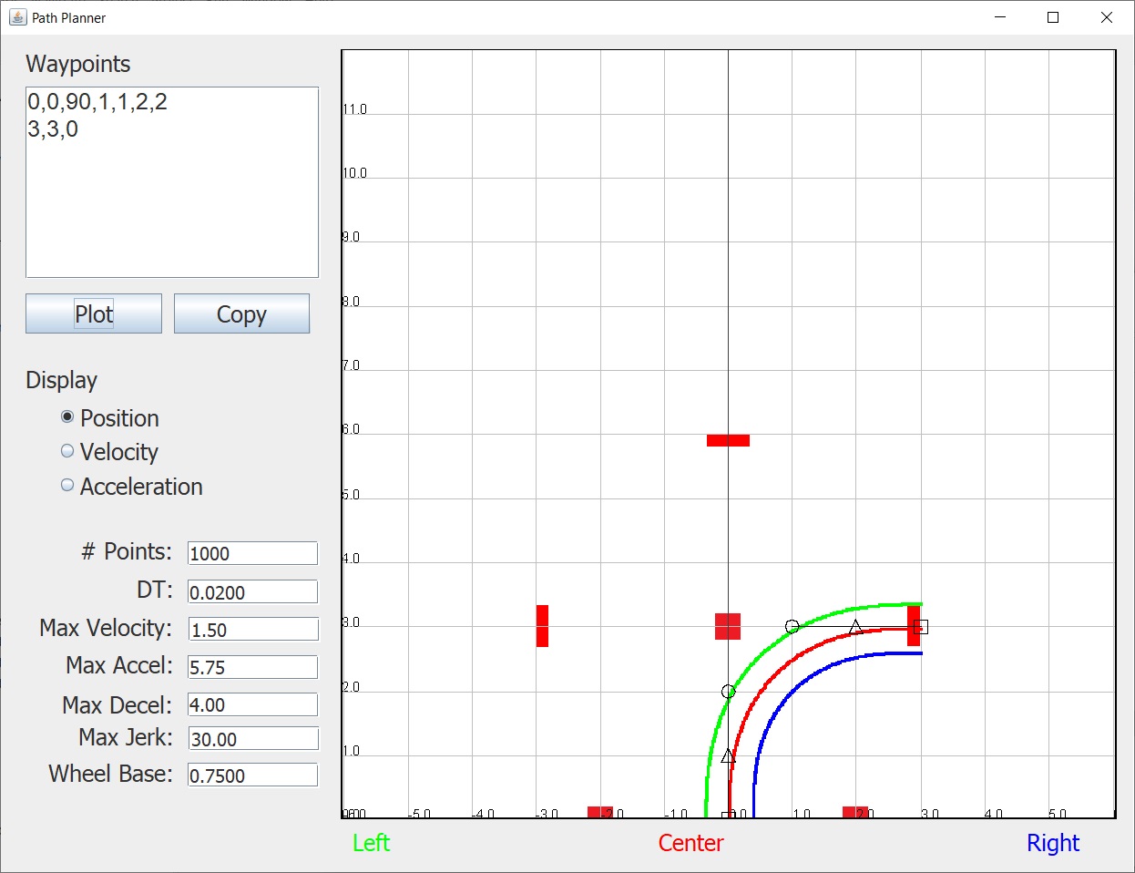
When you start PathPlanner it will display a simple path which goes from (0,0) pointing up (90 degrees) to (3,3) pointing right (0 degrees). The green line represents the path of the left wheel, the red line the center of the robot and the blue line the right wheel.
Note that in the above image I have marked the position of the 6 Bezier control points, P0, P1, P2, P3, P4, and P5. Note that when you use this format, the points P1 and P2 will always be coincident, as will the points P3 and P4. Also the distance the points P1, P2, P3 and P4 are from their respective end points will be automatically calculated based on the length of the path.
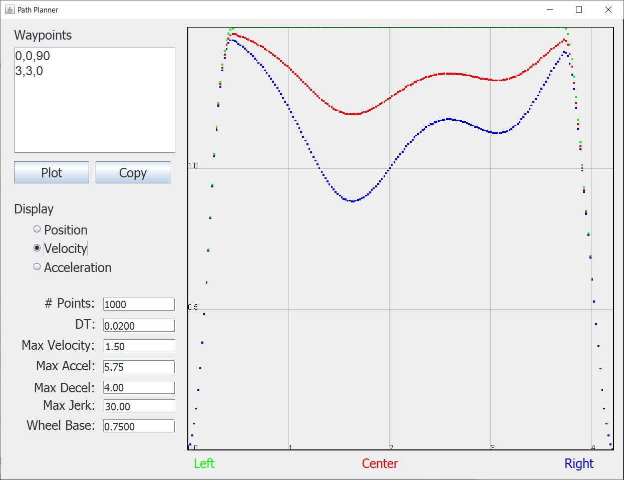
Once you have plotted the curve you can see the required velocities for the center and left and right wheels by clicking the Velocity radio button:
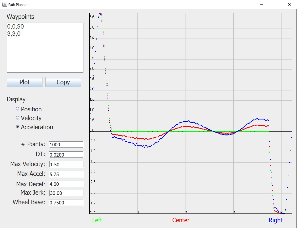
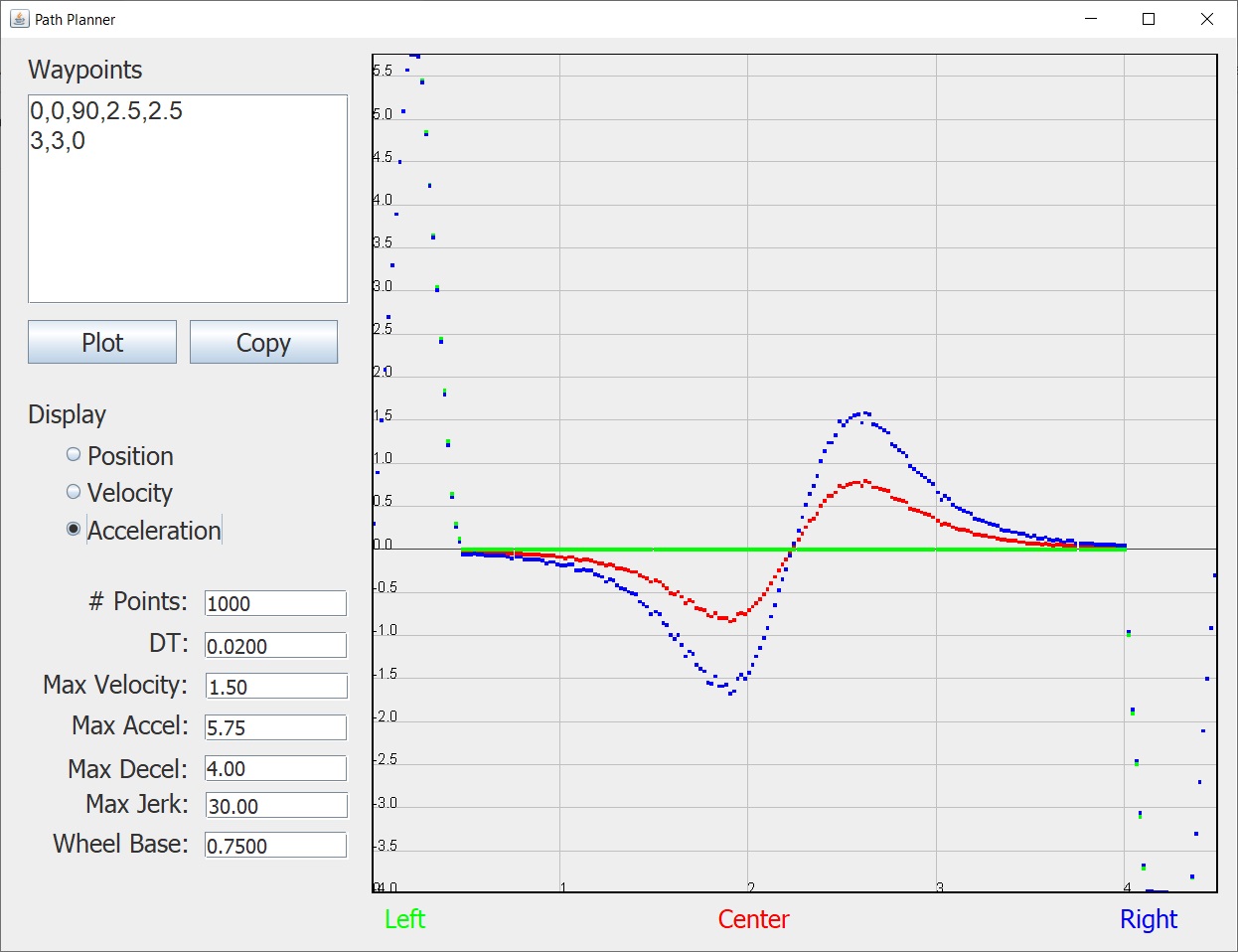
You can also see the acceleration that will be required by clicking the Acceleration radio button:
Now using the basic format to specify the curve endpoints is quick and easy, but we also want to control the position the other four Bezier control points (P1, P2, P3 and P4). In order to maintain the first and second derivatives, these points are constrained to a line that is tangent to the curve at the endpoints. However, the distance of these control points from the endpoints can be controlled and will affect the shape of the curve and the resultant velocities and accelerations required.
For example, we can specify the distance from the endpoints by using 2.5 values for each line instead of the default. If we enter the following into the Waypoints field and display the curve we will see the following:
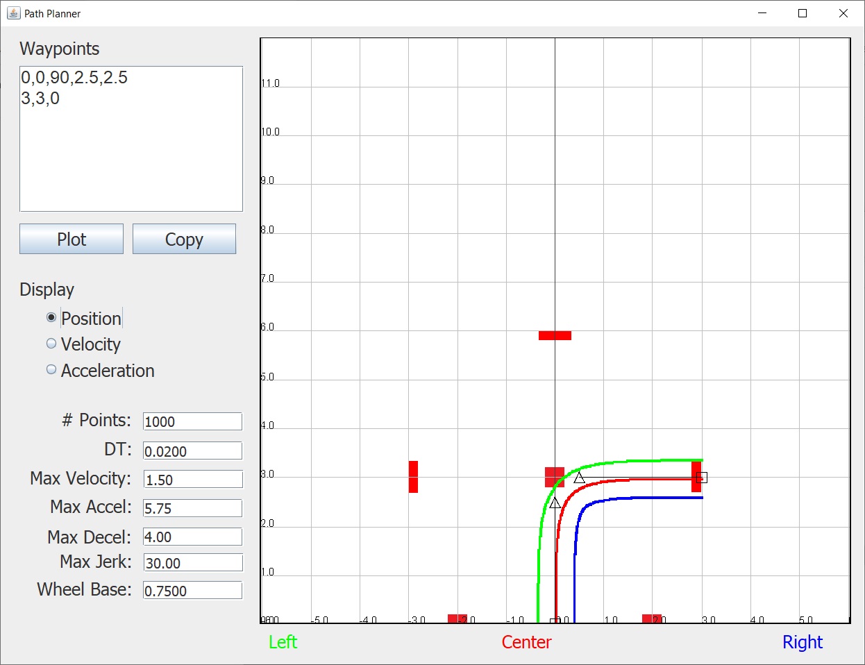
Now you can see that the control points have moved out and this produces a much tighter curve. If we look at the velocity curves we see:
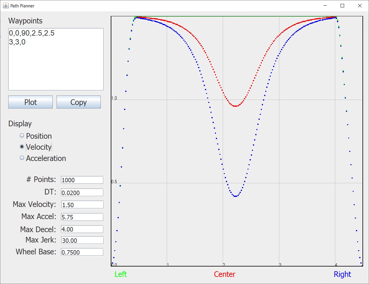
You can see that this tighter curve requires a much greater velocity change for the middle of the path. Looking at the acceleration curves we see:
Now to add additional components to the path, we only need to add additional lines. For example:
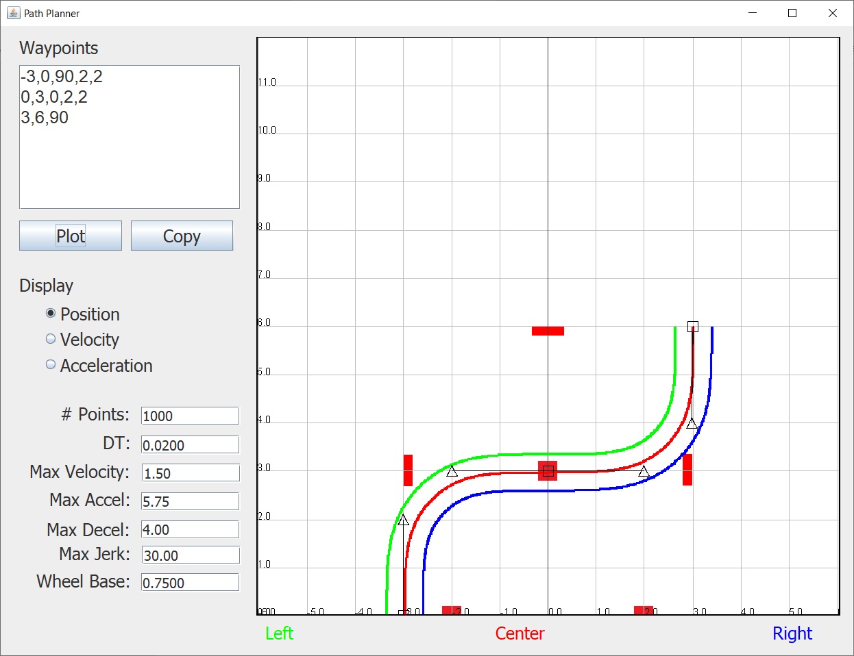
Here the path starts at position (-3,0) moves to position (0,3) and then ends at position (3,6).
Now sometimes it is desirable to use different speeds for different pieces of the path. For example, if you need the robot to execute a particularly tight curve you may need to lower the speed in order to keep the required accelerations within reason. To accommodate this, you can add an optional parameter which specifies the speed for that portion of the path. For example, consider the following:
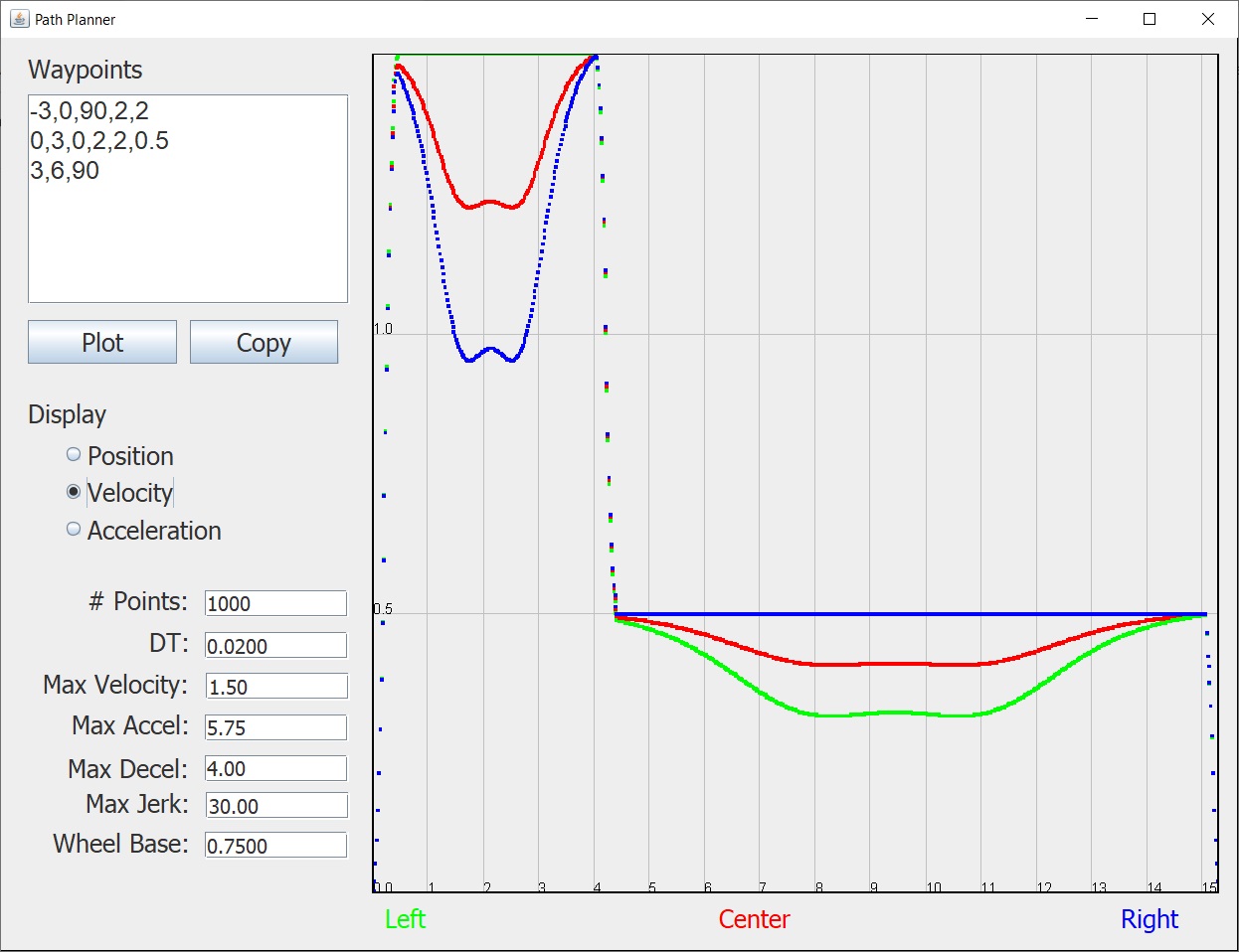
Here we see that the velocity of the robot has been reduced to 0.5 for the second portion of the path.
It is also possible to specify different positions for the P1 and P2 control points as well as different values for the P3 and P4 control points. To do that we add 2 more number to the path line. For example:
As you can see for this new curve, P1 and P2 are no long coincident, as are P3 and P4. Although you can use this to get even greater control over the shape of the curve, we have found that this is probably not necessary.
To summarize, the following are the possible formats that can be used to specify the waypoints:
- x,y,angle
- x,y,angle,speed
- x,y,angle,p12,p34
- x,y,angle,p12,p34,speed
- x,y,angle,p1,p4,p2,p3
- x,y,angle,p1,p4,p2,p3,speed