Path Following – Robotics Programming

Now that we know how to create paths, let’s see if we can get the robot to follow one.

First we need to make some changes to our DriveSubsystem. We are going to use the PurePursuit class to control the motion of the robot so add a PurePursuit variable:

  private final PurePursuit m_pursuit;

1 2	private final PurePursuit m_pursuit;

Now the constructor for PurePursuit requires a function that will set the speed of the left and right wheels in feet/second, so we need to create that:

  public void setSpeedFPS(double leftSpeed, double rightSpeed)
  {
    // Change speed from FPS to -1 to 1 range
    leftSpeed = leftSpeed * k_ticksPerFoot / k_maxSpeed;
    rightSpeed =  rightSpeed * k_ticksPerFoot / k_maxSpeed;

    setSpeed(leftSpeed, rightSpeed);
  }

public void setSpeedFPS(double leftSpeed, double rightSpeed)

{

// Change speed from FPS to -1 to 1 range

leftSpeed = leftSpeed * k_ticksPerFoot / k_maxSpeed;

rightSpeed = rightSpeed * k_ticksPerFoot / k_maxSpeed;

setSpeed(leftSpeed, rightSpeed);

}

Here we are computing the speed as percentage of the max speed by multiplying the speed in feet/second by the ratio of the ticks per foot to the max speed. We can then call our existing setSpeed function.

There is one other change we need to make in addition to creating this setSpeedFPS function. The PurePursuit path follower runs in it’s own thread and will make calls to set the left and right motor speeds via the function you just created. Since these calls will be from a different thread than your normal calls to setPower and setSpeed, we need to enclose any access to the motor classes within a synchronized command. For example, your setPower function should look something like:

  public void setPower(double leftPower, double rightPower)
  {
    synchronized (m_lock)
    {
      m_leftMotor.setControlMode(SmartMotorMode.Power);
      m_rightMotor.setControlMode(SmartMotorMode.Power);

      m_leftMotor.set(leftPower);
      m_rightMotor.set(rightPower);
    }
  }

public void setPower(double leftPower, double rightPower)

{

synchronized (m_lock)

{

m_leftMotor.setControlMode(SmartMotorMode.Power);

m_rightMotor.setControlMode(SmartMotorMode.Power);

m_leftMotor.set(leftPower);

m_rightMotor.set(rightPower);

}

Where you have declared m_lock something like:

  private final Object m_lock = new Object();

1	private final Object m_lock = new Object();

You should have a similar synchronized command in your setSpeed and any other place in your code that you access the instances of your motors.

We are now ready to create an instance if PurePursuit in the constructor of our DriveSubsystem:

    m_pursuit = new PurePursuit(navigator, (l, r) -> { setSpeedFPS(l, r); }, k_purePersuitUpdateRate);
    m_pursuit.enableLogging("/home/pi/logs");

1 2	m_pursuit = new PurePursuit(navigator, (l, r) -> { setSpeedFPS(l, r); }, k_purePersuitUpdateRate); m_pursuit.enableLogging("/home/pi/logs");

Of course we must define k_purePersuitUpdateRate:

 private final static int k_purePursuitUpdateRate  = 50;

1	private final static int k_purePursuitUpdateRate = 50;

Note the call to enableLogging. This allows us to log details about the followed path to a file on the Raspberry Pi, which will allow us to study how well the robot is following the path.

Finally we will need a few functions to control the path following from our commands:

  /*
   * This function loads a specified path and the starts the following
   */
  public void startPath(Path path, boolean isReversed, boolean isExtended) {
    m_pursuit.loadPath(path, isReversed, isExtended);
    m_pursuit.startPath();
  }

  /*
   * This function ends the currently followed path (if any)
   */
  public void endPath() {
    m_pursuit.stopFollow();
  }

  /*
   * This function returns true if the current path has completed
   */
  public boolean isPathFinished() {
    return (m_pursuit.isFinished());
  }

* This function loads a specified path and the starts the following

public void startPath(Path path, boolean isReversed, boolean isExtended) {

m_pursuit.loadPath(path, isReversed, isExtended);

m_pursuit.startPath();

}

* This function ends the currently followed path (if any)

public void endPath() {

m_pursuit.stopFollow();

}

* This function returns true if the current path has completed

public boolean isPathFinished() {

return (m_pursuit.isFinished());

}

Before we create our first follow path command, we need to do one more thing. The Pure Pursuit path following has a number of tunable parameters. While it is possible to specify a different set of parameters for each path, it is useful to set up a set of defaults that are used for each new path we create. You do this in the RobotContainer’s constructor by adding the following. Be sure to place these lines before the call to configureButtonBindings().

    Pathfinder.setDefaultLookAheadTime(k_lookAheadTime);
    Pathfinder.setDefaultMinLookAheadDistance(k_minLookAheadDist);
    Pathfinder.setDefaultMaxSearchTime(k_maxSearchTime);
    Pathfinder.setDefaultMinSpeed(k_minSpeed);
    Pathfinder.setDefaultExtendedLookAheadDistance(k_extendedLookAhead);
    Pathfinder.SetDefaultCurvatureAdjust(k_curvatureAdjust);

Pathfinder.setDefaultLookAheadTime(k_lookAheadTime);

Pathfinder.setDefaultMinLookAheadDistance(k_minLookAheadDist);

Pathfinder.setDefaultMaxSearchTime(k_maxSearchTime);

Pathfinder.setDefaultMinSpeed(k_minSpeed);

Pathfinder.setDefaultExtendedLookAheadDistance(k_extendedLookAhead);

Pathfinder.SetDefaultCurvatureAdjust(k_curvatureAdjust);

Where we have defined the constants as:

  private static final double k_lookAheadTime = 0.75;		// Time along the path of the next target point	
  private static final double k_minLookAheadDist = 0.6;		// Minimum allowed look ahead distance (overrides look ahead time if necessary)
  private static final double k_maxSearchTime = 1;		// Max time along the path to search for the closest point to the current position
  private static final double k_minSpeed = 0.50;			// Minimum allowed speed
  private static final double k_extendedLookAhead = .75;	// Distance to extend path if m_isExtended is true
  private static final double k_curvatureAdjust = 1.0;		// Adjusts the curvature to make the path following more or less aggressive

private static final double k_lookAheadTime = 0.75; // Time along the path of the next target point

private static final double k_minLookAheadDist = 0.6; // Minimum allowed look ahead distance (overrides look ahead time if necessary)

private static final double k_maxSearchTime = 1; // Max time along the path to search for the closest point to the current position

private static final double k_minSpeed = 0.50; // Minimum allowed speed

private static final double k_extendedLookAhead = .75; // Distance to extend path if m_isExtended is true

private static final double k_curvatureAdjust = 1.0; // Adjusts the curvature to make the path following more or less aggressive

Let’s take a look at what each of these values mean. See the documentation for PathFinder for further information.

Look Ahead Time – This is the time that Pure Pursuit looks ahead on the path to find the point at which to steer. We will use a default of 0.75 seconds along the path.
Minimum Look Ahead Distance – If the distance computed by using the Look Ahead Time is less than this minimum, then this value will be used instead. We will set this minimum to default to 0.6 feet.
Maximum Search Time – On Each update, the path will be searched for the point on the path that is closest to the robot’s current position. To avoid problems when the robot loops back on it’s own path, this value specifies the maximum time to look ahead for the closest point. We will set this to default to 0.25 seconds along the path.
Minimum Speed – This value specifies the minimum speed for the robot that is needed to keep the robot from stalling. We will set this value 0.50 feet/second.
Extended Look Ahead – This value specifies the amount to extend the path for navigation purposes if the isExtended flag is set to true on the call to loadPath. Note that this extension is used for navigation purposes only and the robot will still stop at the final ending point. We will set this to default to 0.75 feet.
Curvature Adjust – This value is used to force the robot to more (or less) aggressively steer toward the target point. A value of 1 will use the curvature that is computed by the Pure Pursuit algorithm. A value greater than 1 will cause the robot to steer more aggressively towards that point and a value less than 1 will cause the robot to steer less aggressively. We set this to the default of 1.0.

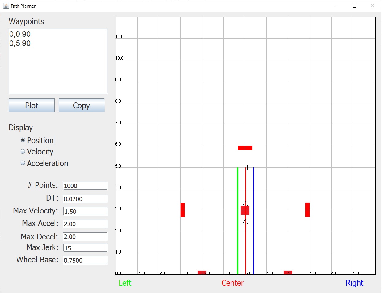
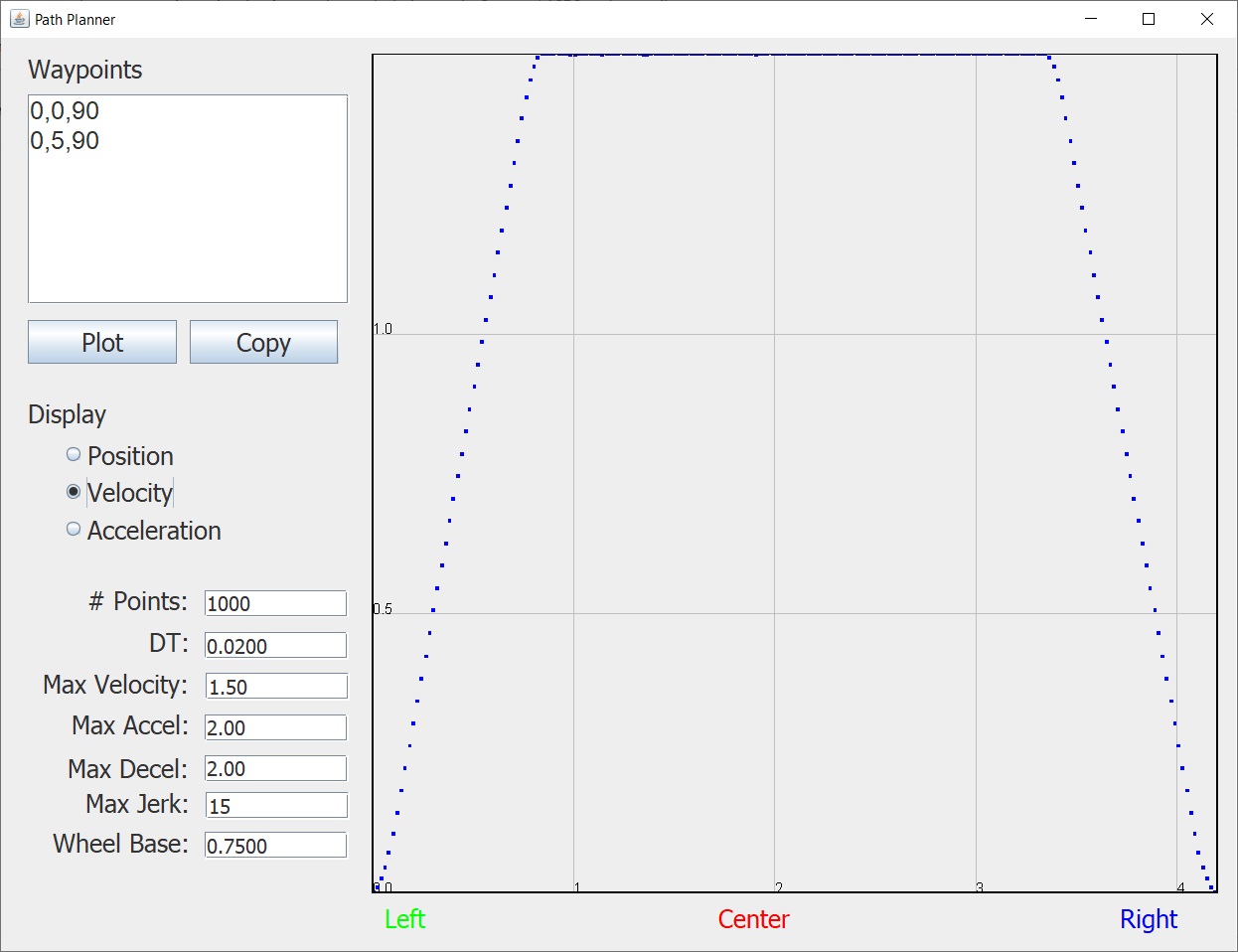
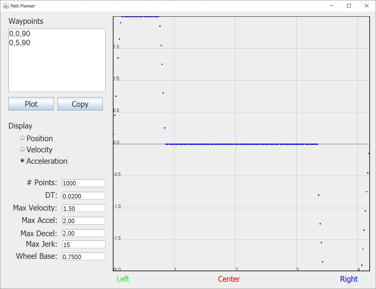
We are now ready to create our first path following command. For this command we will instruct the robot to drive forward 5 feet. The first thing to do is to create the path in the PathPlanner program. Graphing the position, velocity and acceleration we see the following:

The structure of all of your path following commands will be similar. Below is my example of a command to drive forward 5 feet. Note that I am placing all of my pursuit commands into a purePursuit subfolder of commands just to keep them organized.

package robot.commands.purePursuit;

import edu.wpi.first.wpilibj2.command.CommandBase;
import pathfinder.Pathfinder;
import pathfinder.Pathfinder.Path;
import pathfinder.Pathfinder.Waypoint;
import robot.subsystems.DriveSubsystem;
import robotCore.Logger;
import robotCore.Navigator;

/**
 * An example command that uses an example subsystem.
 */
public class Drive5ftCommand extends CommandBase {
  private final DriveSubsystem m_subsystem;
  private final Path m_path;
  private final Navigator m_navigator;

  private static final int k_nPoints = 1000;
  private static final double k_dt = 0.020000;
  private static final double k_maxSpeed = 1.500000;
  private static final double k_maxAccel = 2.000000;
  private static final double k_maxDecl = 2.000000;
  private static final double k_maxJerk = 15.000000;
  private static final double k_wheelbase = 0.750000;
  /*
  0,0,90
  0,5,90
  */
  private static final Waypoint[] k_path = {
      new Waypoint(0, 0, Math.toRadians(90)),
      new Waypoint(0, 5, Math.toRadians(90))
  };

  /**
   * Creates a new Drive5ftCommand.
   *
   * @param subsystem The subsystem used by this command.
   */
  public Drive5ftCommand(DriveSubsystem subsystem, Navigator navigator) {
    Logger.log("Drive5ftCommand", 3, "Drive5ftCommand()");

    m_subsystem = subsystem;
    m_navigator = navigator;
    // Use addRequirements() here to declare subsystem dependencies.
    addRequirements(m_subsystem);

    m_path = Pathfinder.computePath(k_path, k_nPoints, k_dt, k_maxSpeed, k_maxAccel, k_maxDecl, k_maxJerk, k_wheelbase);
  }

  // Called when the command is initially scheduled.
  @Override
  public void initialize() {
    Logger.log("Drive5ftCommand", 2, "initialize()");

    /*
     * We reset the robot to the starting position and orientation.
     *  Note that if you end up stringing multiple path following commands together using a group,
     *  you should do this reset ONLY for the first command int the group
     */
    m_navigator.reset(90, 0, 0);

    // Load and start the path following
    m_subsystem.startPath(m_path, false, true, true);
  }

  // Called every time the scheduler runs while the command is scheduled.
  @Override
  public void execute() {
    Logger.log("Drive5ftCommand", -1, "execute()");

    // The path following is handled by the PurePursuit class so we don't need to do anything here
  }

  // Called once the command ends or is interrupted.
  @Override
  public void end(boolean interrupted) {
    Logger.log("Drive5ftCommand", 2, String.format("end(%b)", interrupted));

    // End the path following when the command ends.
    m_subsystem.endPath();
  }

  // Returns true when the command should end.
  @Override
  public boolean isFinished() {
    Logger.log("Drive5ftCommand", -1, "isFinished()");

    // Return true if the path has completed
    return m_subsystem.isPathFinished();
  }
}

package robot.commands.purePursuit;

import edu.wpi.first.wpilibj2.command.CommandBase;

import pathfinder.Pathfinder;

import pathfinder.Pathfinder.Path;

import pathfinder.Pathfinder.Waypoint;

import robot.subsystems.DriveSubsystem;

import robotCore.Logger;

import robotCore.Navigator;

/**

* An example command that uses an example subsystem.

public class Drive5ftCommand extends CommandBase {

private final DriveSubsystem m_subsystem;

private final Path m_path;

private final Navigator m_navigator;

private static final int k_nPoints = 1000;

private static final double k_dt = 0.020000;

private static final double k_maxSpeed = 1.500000;

private static final double k_maxAccel = 2.000000;

private static final double k_maxDecl = 2.000000;

private static final double k_maxJerk = 15.000000;

private static final double k_wheelbase = 0.750000;

0,0,90

0,5,90

private static final Waypoint[] k_path = {

new Waypoint(0, 0, Math.toRadians(90)),

new Waypoint(0, 5, Math.toRadians(90))

};

/**

* Creates a new Drive5ftCommand.

* @param subsystem The subsystem used by this command.

public Drive5ftCommand(DriveSubsystem subsystem, Navigator navigator) {

Logger.log("Drive5ftCommand", 3, "Drive5ftCommand()");

m_subsystem = subsystem;

m_navigator = navigator;

// Use addRequirements() here to declare subsystem dependencies.

addRequirements(m_subsystem);

m_path = Pathfinder.computePath(k_path, k_nPoints, k_dt, k_maxSpeed, k_maxAccel, k_maxDecl, k_maxJerk, k_wheelbase);

}

// Called when the command is initially scheduled.

@Override

public void initialize() {

Logger.log("Drive5ftCommand", 2, "initialize()");

* We reset the robot to the starting position and orientation.

* Note that if you end up stringing multiple path following commands together using a group,

* you should do this reset ONLY for the first command int the group

m_navigator.reset(90, 0, 0);

// Load and start the path following

m_subsystem.startPath(m_path, false, true, true);

}

// Called every time the scheduler runs while the command is scheduled.

@Override

public void execute() {

Logger.log("Drive5ftCommand", -1, "execute()");

// The path following is handled by the PurePursuit class so we don't need to do anything here

}

// Called once the command ends or is interrupted.

@Override

public void end(boolean interrupted) {

Logger.log("Drive5ftCommand", 2, String.format("end(%b)", interrupted));

// End the path following when the command ends.

m_subsystem.endPath();

}

// Returns true when the command should end.

@Override

public boolean isFinished() {

Logger.log("Drive5ftCommand", -1, "isFinished()");

// Return true if the path has completed

return m_subsystem.isPathFinished();

}

Lets take a look at a couple of features of this command. First we have the following lines which defines the path.

  private static final int k_nPoints = 1000;
  private static final double k_dt = 0.020000;
  private static final double k_maxSpeed = 1.500000;
  private static final double k_maxAccel = 2.000000;
  private static final double k_maxDecl = 2.000000;
  private static final double k_maxJerk = 15.000000;
  private static final double k_wheelbase = 0.750000;
  /*
  0,0,90
  0,5,90
  */
  private static final Waypoint[] k_path = {
      new Waypoint(0, 0, Math.toRadians(90)),
      new Waypoint(0, 5, Math.toRadians(90))
  };

private static final int k_nPoints = 1000;

private static final double k_dt = 0.020000;

private static final double k_maxSpeed = 1.500000;

private static final double k_maxAccel = 2.000000;

private static final double k_maxDecl = 2.000000;

private static final double k_maxJerk = 15.000000;

private static final double k_wheelbase = 0.750000;

0,0,90

0,5,90

private static final Waypoint[] k_path = {

new Waypoint(0, 0, Math.toRadians(90)),

new Waypoint(0, 5, Math.toRadians(90))

};

These numbers come directly from the PathPlanner program. Note, however, you do not need to type these in. If you click the Copy button in PathPlanner, these lines will be copied to the clipboard and you can just paste them into your program.

In our constructor we create the path by calling the computePath function of the Pathfinder class.

    m_path = Pathfinder.computePath(k_path, k_nPoints, k_dt, k_maxSpeed, k_maxAccel, k_maxDecl, k_maxJerk, k_wheelbase);

1 2	m_path = Pathfinder.computePath(k_path, k_nPoints, k_dt, k_maxSpeed, k_maxAccel, k_maxDecl, k_maxJerk, k_wheelbase);

In our initialize function we reset the robot to it’s starting position (0,0) and starting yaw (angle) of 90 degrees. Note that if we later make a command which consists of multiple path following commands we only want to do this reset in the first of the set.

Also in our initialize function we start the path following by calling the startPath function of our DriveSubsystem.

    m_subsystem.startPath(m_path, false, true, true);

1 2	m_subsystem.startPath(m_path, false, true, true);

Note that the first Boolean parameter controls whether the robot will move forward (false) or backwards (true). We want to go forward so this is set to false. Setting the second Boolean parameter to true will help keep the robot from turning as it approaches it’s destination. The last parameter controls whether the navigator will be automatically reset to the starting position and angle for the path. We always want to set this to true for the first path. If we have it follow multiple paths, we will set it to false for the subsequent paths.

In the end function we end the path following by calling the endPath function of our DriveSubsystem.

    m_subsystem.endPath();

1	m_subsystem.endPath();

Finally in the isFinished function we return whether the path is complete by calling the isPathFinished function of our DriveSubsystem.

    return m_subsystem.isPathFinished();

1	return m_subsystem.isPathFinished();

Now connect this command to a button (using whenPressed) and run your program. When you press the button, the robot should drive forward 5 feet and then stop.

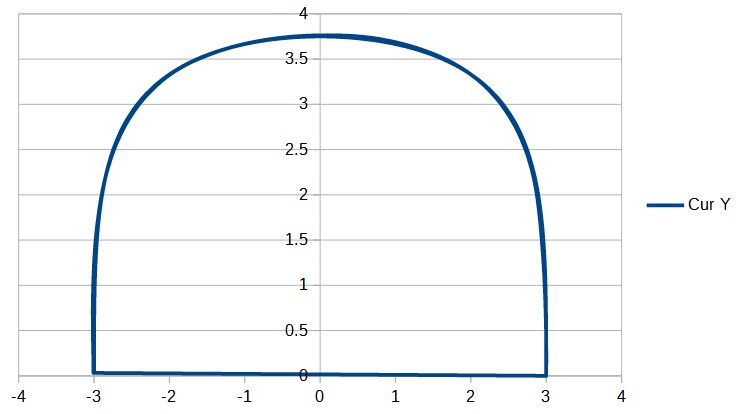
Now try creating a more complicated path that drives the robot from (3,0) at 90 degrees to (-3,0) at -90 degrees. You can construct the path using a single Bezier curve like this:

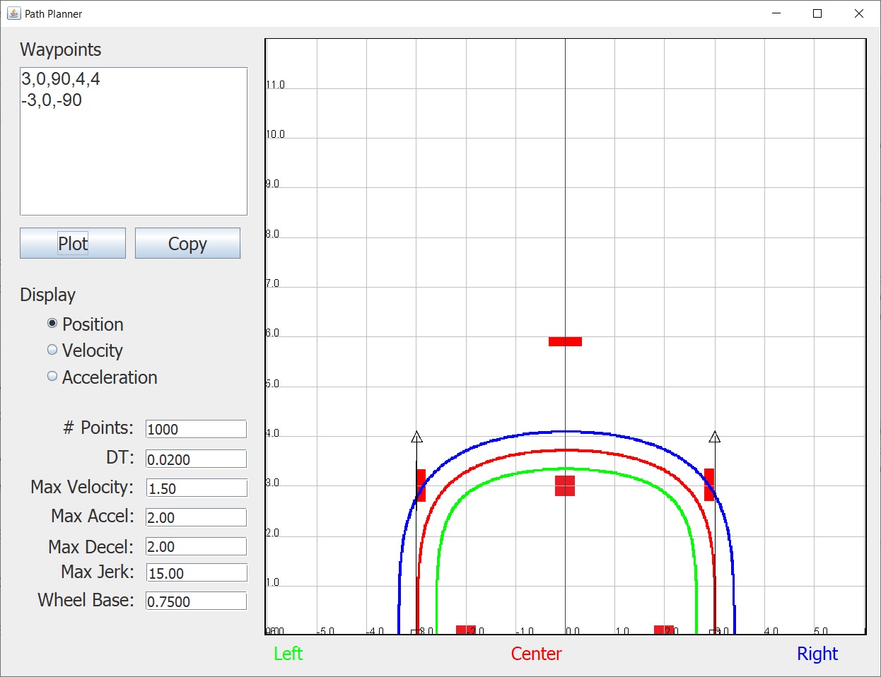
Or you can connect two Bezier curves like this:

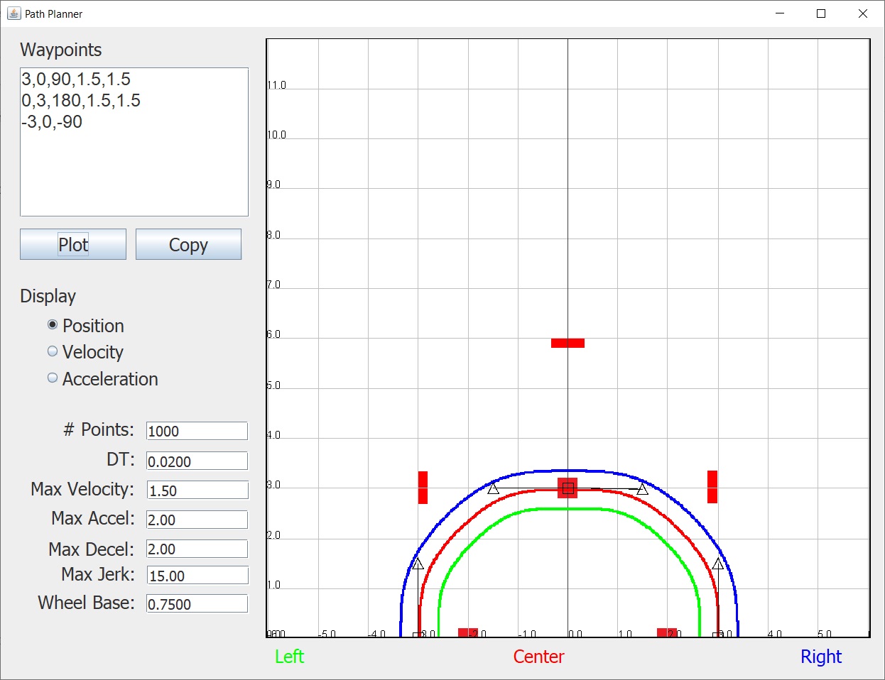
Note that if we need the robot to go through the point (0,3) then it is easier to do it with 2 curves rather than one, although it would still be possible with one by changing the Bezier control points.

Create a new command called SemiCircleCommand that implements this path. The easiest way is to copy the Drive5ftCommand and replace the path with your new one. Remember that you can use the Copy button in the PathPlanner and paste that code into your command. When you have finished run your program and verify that the robot drives the correct path.

Now before we move on, I want to introduce you to a tool that will let you examine the path the robot took in detail. The way we have configured PurePursuit, it will log detailed information about the path following to a logs folder in the home directory of the pi.

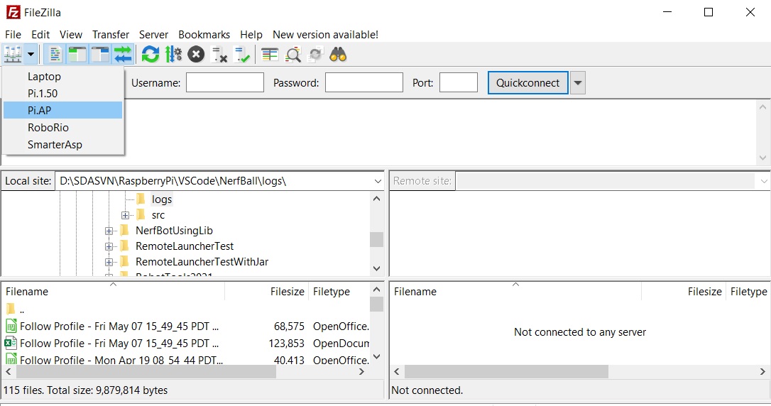
To examine this data, we will first need to upload the log file to our compute. For this we will us the FTP program FileZilla. Then connect to the pi by selecting the Pi.AP option from the dropdown shown below:

Create a logs subfolder in your robot project folder and then in the left Local Site pane navigate to that folder. In the right Remote Site pane, navigate to the logs folder as shown below:

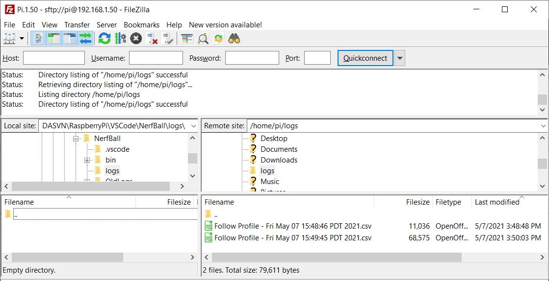
Click on the Last modified header of the right pane to show the most recent file first. Then double click on the most recent file to copy it to the logs folder on your computer.

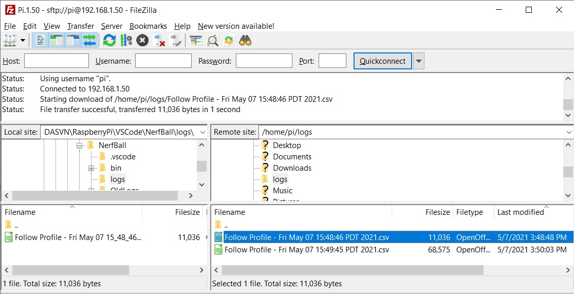
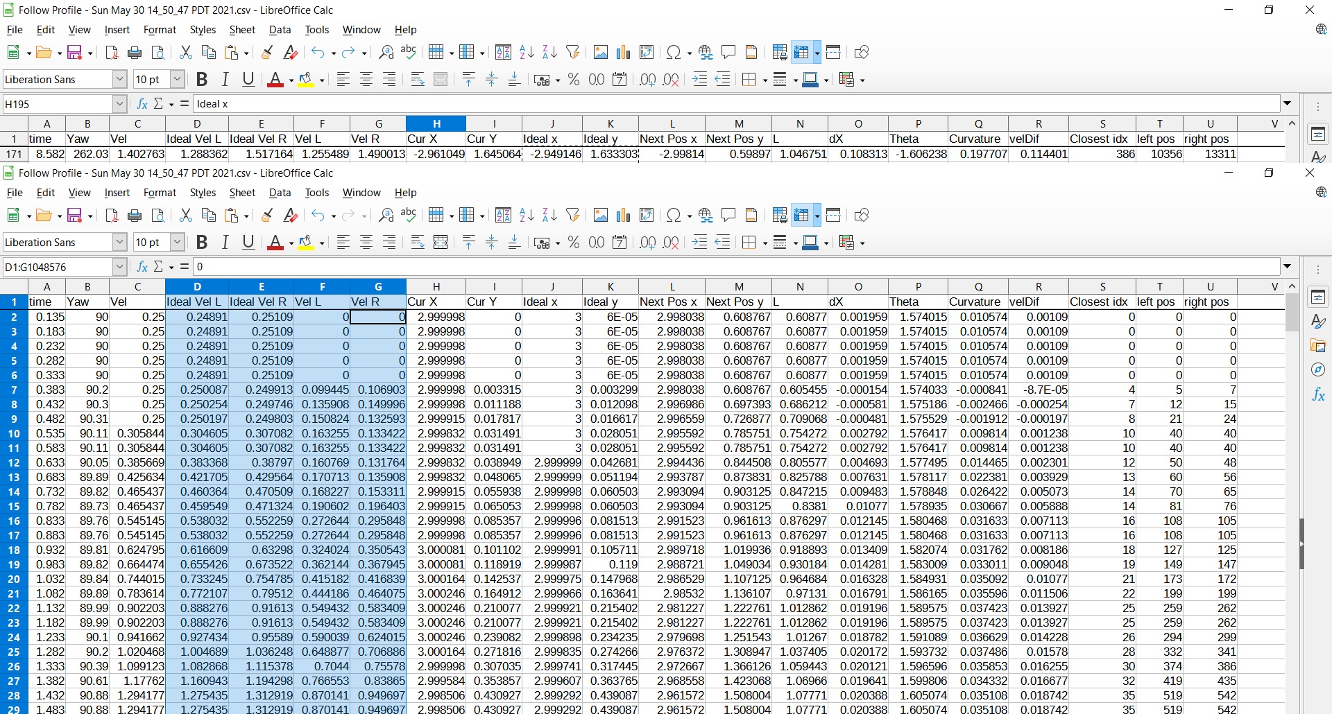
Then right click on the file in the left pane and choose Open. This will open the file in LibreCalc.

First we will compare the Ideal left and right velocities to the Actual left and right velocities. Select the columns D, E, F, and G as shown.

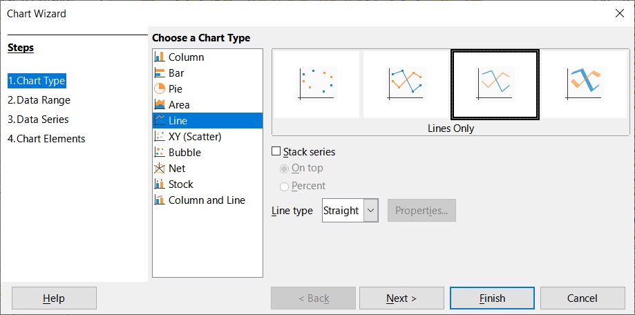
Then create a chart choosing Line/Lines Only options:

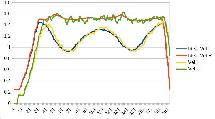
This will produce a graph showing the Ideal and Actual velocity of both wheels and we can see how closely the velocities are being matched.

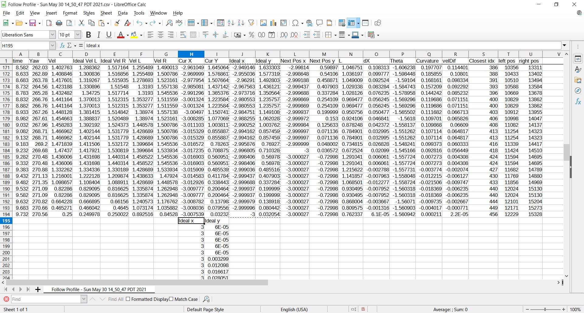
Finally, we can plot the Actual path to the Ideal path to see how well they match as well. Do do this in LibreCalc, we will first need to select all of the Ideal x and y data (columns J and K) and past it onto the end of the Actual x and y data (columns H and I) as shown:

Then select columns H and I and create a chart, this time choosing XY (Scatter):

As a final exercise for this section, create a command to follow the following path:

Next: Final Challenge